Surprising but ineffectual. How a significant p-value can be practically unimportant?
When p < 0.001 means almost nothing — a Football case study in why statistical significance isn’t practical importance.
Football Analytics
Author
Murat Seyhan
Published
March 21, 2026
If you’ve spent any time around Turkish football discourse — or really, football discourse anywhere — you know the consensus. Big teams press. Big teams don’t give the ball to the opponent and sit back. That is practically a law of nature in our football culture. And it’s not just a Turkish thing — since Klopp turned Liverpool into European champions with Gegenpressing, every post-match panel everywhere seems to agree. “They pressed high,”“they won the ball back in dangerous areas,”“their intensity off the ball was the difference.” It’s become the thing every pundit says when a team plays well.
I get the appeal. Pressing looks like effort, like intent, like a team that wants it more. And the data seems to back it up at the first sight?
What Is PPDA and Why Do We Care?
Football analytics has a pretty clean way of measuring pressing intensity: PPDA, or Passes Per Defensive Action — a metric originally developed by Colin Trainor, who deserves a lot of credit for giving the analytics community a simple but powerful tool to quantify something that used to be purely vibes-based. The idea is intuitive — you count how many passes the opposing team completes before your team does something about it. A tackle, an interception, a foul. Low PPDA means you’re disrupting them quickly. High PPDA means you’re sitting back and letting them circulate the ball. The lower the number, the harder the squeeze.
It’s an elegant metric, and it captures something real about how teams defend. The question I wanted to explore isn’t about PPDA itself — it’s about what happens when we take a metric like this, run a statistical test, get a shiny p-value, and stop thinking too early.
To test whether pressing translates into results, I pulled StatsBomb event data for all five major European leagues from the 2015/16 season — Premier League, La Liga, Serie A, Bundesliga, and Ligue 1. That’s 1,823 matches, 3,646 team-match observations. For each one, I calculated PPDA from raw event-level data (excluding set-piece passes) and recorded the match outcome in points — 3 for a win, 1 for a draw, 0 for a loss.
The question is straightforward. Does pressing harder lead to more points?
Let’s test it.
NoteNotes on the data and PPDA calculation
PPDA is calculated from StatsBomb event-level data as: (opponent open-play passes in the attacking zone) / (tackles + interceptions + fouls in the defensive zone). Set-piece passes (goal kicks, throw-ins, free kicks, corners, kick-offs) are excluded from the numerator — StatsBomb logs these as type=="Pass" with a pass_type field, but Opta’s original PPDA formulation treats them separately. This exclusion brings league averages in line with published benchmarks (~10–13 range).
The zone thresholds follow the convention: defending team actions at loc_x > 48 (own half), opponent passes at loc_x < 72. Each match produces two rows — one per team.
Matches: 1,823
Team-match observations: 3,646
Leagues: 1. Bundesliga, La Liga, Ligue 1, Premier League, Serie A
The Hypothesis Test: The p-Value Speaks
Here’s the formal setup:
Null hypothesis H₀: there’s no difference in match points between teams that press aggressively (PPDA below 10) and teams that sit back (PPDA above 15).
Alternative hypothesis H₁: aggressive pressing teams earn more points.
The groups: 1,496 observations with aggressive pressing, 905 with passive pressing. Let’s run a two-sample Welch’s t-test.
# Filter the dataframe to get points for teams with aggressive pressing (PPDA < 10)agg = df[df['ppda'] <10]['points']# Filter the dataframe to get points for teams with passive pressing (PPDA > 15)pas = df[df['ppda'] >15]['points']# Perform Welch's t-test to compare the means of the two groups (unequal variances assumed)t_stat, p_val = stats.ttest_ind(agg, pas, equal_var=False)# Print summary statistics and test resultsprint(f'Aggressive pressing (PPDA < 10): n = {len(agg)}, mean = {agg.mean():.3f} pts/match')print(f'Passive pressing (PPDA > 15): n = {len(pas)}, mean = {pas.mean():.3f} pts/match')print(f'\nWelch\'s t = {t_stat:.2f}, p = {p_val:.6f}')
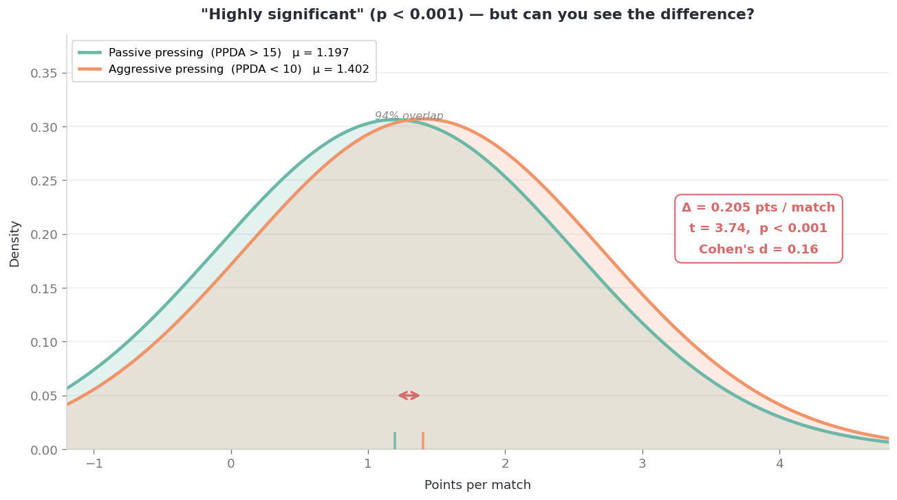
Aggressive pressing (PPDA < 10): n = 1496, mean = 1.402 pts/match
Passive pressing    (PPDA > 15): n = 905, mean = 1.197 pts/match

Welch's t = 3.74,  p = 0.000188
Highly significant. That simply means; If pressing truly had no effect on match outcomes, you’d see a difference this large less than 0.02% of the time just by chance. The null hypothesis looks implausible. And I think this is where most people’s intuitive reaction kicks in — the gut says “I knew it, pressing works.”
That’s a very natural response. Our brain is a causality machine, and when a test confirms something we already believed, we accept it fast. p < 0.001? Done. Moving on.
And honestly, in a lot of real-world scenarios, this is exactly how it plays out. In corporate analytics, in quick-turnaround decisions, in situations where you need a fast read on whether something matters — the p-value has become something like fast food for statistical thinking. You order it, you get your answer in seconds, and you move on to the next thing. The person making the call sees “significant” and acts. Nobody stops to check how big the effect actually is. Not because they’re lazy — because the workflow doesn’t always leave room for it, and because the word “significant” feels like it already answered the question.
But it didn’t. The p-value told us this result would be surprising if there were no effect at all. It said literally nothing about how big that effect is. And the size of the effect is the thing that actually determines whether you should care.
What the p-Value Hides
Let’s report some of the statistical regularities behind our data.
raw effect in context
aggressive (PPDA < 10) vs passive (PPDA > 15) points-per-match gap
this is the difference in group means, the practical point delta you’d feel on the pitch
pooled standard deviation
combines both groups’ spread into a single scale (for effect-size normalization)
gives us a stable denominator for Cohen’s d
Cohen’s d effect size
mean difference divided by pooled sd
unitless, comparable across studies
usual benchmarks: 0.2 small, 0.5 medium, 0.8 large
probability of superiority (P(superiority))
chance a random aggressive-team result beats a random passive-team result
derived from Cohen’s d under normality assumptions
50% is coin flip, >50% means the aggressive side tends to edge out
distribution overlap
percent overlap of two normalized outcome curves
close to 100% means almost no practical separation, even when p is tiny
These are the real “magnitude” diagnostics that tell whether a significant p-value is also meaningful in practice.
Mean difference:       0.205 points/match
Cohen's d:             0.16
P(superiority):        54%  (coin flip = 50%)
Distribution overlap:  94%
The actual mean difference between the two groups? 0.205 points per match. Cohen’s d comes out to 0.16 — below the threshold of what’s typically called a “small” effect. Most would put this in the negligible range.
Now I want you to feel what that means in practice. If you randomly picked one match from each group and asked “which one produced more points?”, the aggressive pressing match would come out ahead 54% of the time. That’s 4 percentage points above a coin flip. The two distributions overlap by 94%. If someone mixed the results from both groups together without labels, you could not sort them back.
The p-value said “significant.” The effect size tells a very different story — the effect exists, sure, but you’d have a hard time spotting it with your bare eyes.
Why Was the p-Value So Small Then?
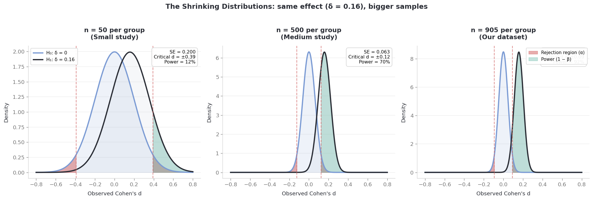
A p-value is a function of two things: the effect size and the sample size. The t-statistic:
t = (mean difference) / (standard error)
As your sample grows, the standard error shrinks. With nearly 2,400 observations per group, even a whisper of a difference will produce a large t-statistic. The math doesn’t care if the difference is meaningful — it only cares that it’s detectable.
See two bell curves above. The sampling distribution under the null (no effect) and the one under the alternative (a small effect exists). When the sample is small, both curves are wide and overlap almost completely. The test can’t tell them apart. As n gets bigger, both curves narrow, their peaks sharpen, and eventually even the tiniest gap crosses the significance threshold.
Same effect — the exact same 0.205-point difference — tested at different sample sizes:
print(f'{"n (per group)":>14s}{"p-value":>10s} Significant?')print(f'{"-"*14}{"-"*10}{"-"*12}')for n in [50, 200, 500, 1000, 2400]: se = pooled_sd * np.sqrt(2/n) t = mean_diff / se p =2* (1- stats.t.cdf(abs(t), df=2*n-2)) p_str =f'{p:.3f}'if p >=0.001else'< 0.001' sig ='★ Yes'if p <0.05else' No'print(f'{n:>14,d}{p_str:>10s}{sig}')
 n (per group)     p-value  Significant?
--------------  ----------  ------------
            50       0.432    No
           200       0.116    No
           500       0.013  ★ Yes
         1,000     < 0.001  ★ Yes
         2,400     < 0.001  ★ Yes
Look at this table carefully. The effect hasn’t changed. The same trivial difference sits at every row. At n = 50 the p-value says “nope, not significant.” At n = 2,400 it calls the same difference “highly significant.” The p-value didn’t discover something important — it just accumulated enough data to detect something trivial.
This is not a flaw in the p-value. It’s doing exactly what it was designed to do. The problem starts when “surprising” gets interpreted as “important.” The test gained the power to detect a negligible effect. Detecting it doesn’t make it matter.
The Size Matters, Actually…
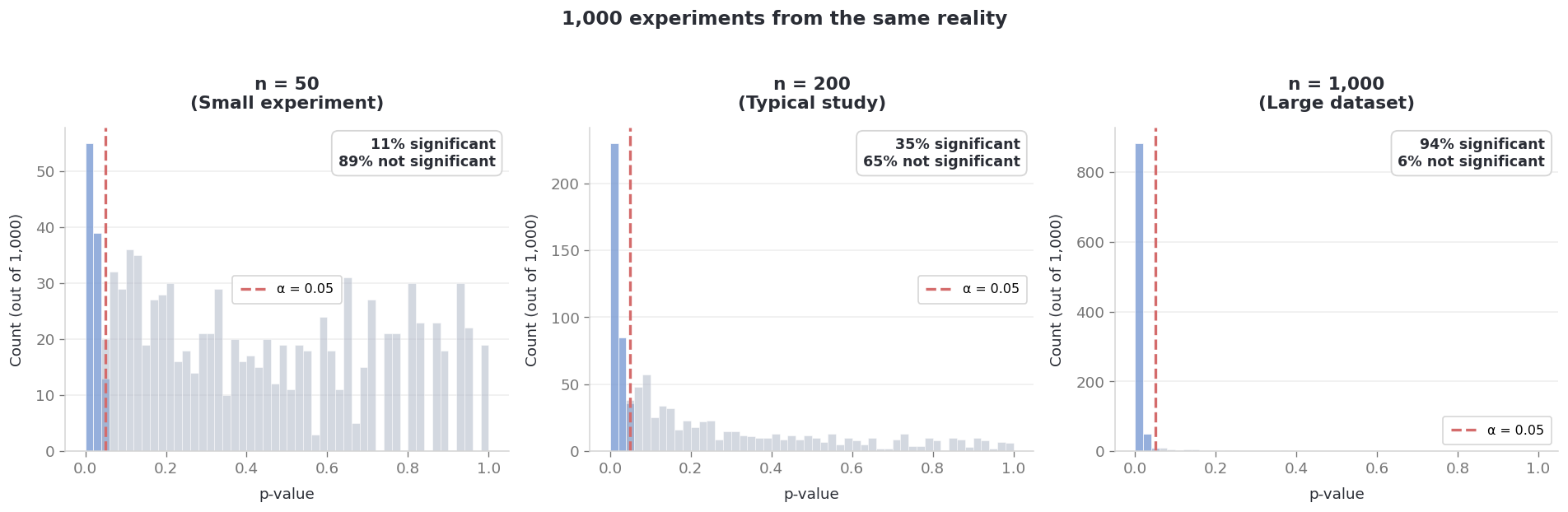
Let’s resample the dataset 1,000 times at three different sample sizes — drawing random subsets and running a fresh t-test each time. Same underlying reality, same true effect. Here’s what happened:
At n = 50 per group, only 11% of experiments crossed the significance threshold. At n = 200, it was 36%. At n = 1,000, it jumped to 93%.
Think about that for a second. Two researchers studying the exact same question with n = 200 would disagree on “significance” more often than they’d agree. Same truth, same test, wildly different conclusions — depending entirely on how many observations happened to land in their sample.
A single p-value is not a reliable foundation for a decision. It’s one draw from a noisy distribution.
What Would Pressing Actually Buy Your Team?
So far we’ve established that the effect exists but is small. Now the question every decision-maker should actually ask: what would acting on this get us in practice?
The comparison I showed you earlier — aggressive pressers vs. passive ones — is misleading, because it compares fundamentally different teams. Barcelona’s PPDA is low and their points tally is high, but that doesn’t mean pressing caused the points. Good teams press because they have better players, more possession, more chances to win the ball back high up the pitch. The question isn’t whether Barcelona earns more points than a relegation candidate. The question is: if your team — your specific team — pressed harder than usual, would you get more points?
This is what a within-team analysis answers. For each team, I calculated how much their PPDA deviated from their own season average in each match, and whether that deviation predicted more or fewer points.
df['ppda_dm'] = df['ppda'] - df.groupby(['competition','team'])['ppda'].transform('mean')df['pts_dm'] = df['points'] - df.groupby(['competition','team'])['points'].transform('mean')slope, _, r_w, p_w, _ = stats.linregress(df['ppda_dm'], df['pts_dm'])print(f'Within-team correlation: r = {r_w:.4f}, R² = {r_w**2:.4f}, p = {p_w:.4f}')print(f'Slope: {slope:.5f} points per 1-unit PPDA change')print(f'\nWhat does a tactical shift actually buy you?')print(f' Lower PPDA by 2 → {slope *-2*38:+.2f} extra points/season')print(f' Lower PPDA by 5 → {slope *-5*38:+.2f} extra points/season')
Within-team correlation:  r = -0.0429,  R² = 0.0018,  p = 0.0096
Slope: -0.00855 points per 1-unit PPDA change

What does a tactical shift actually buy you?
  Lower PPDA by 2  → +0.65 extra points/season
  Lower PPDA by 5  → +1.63 extra points/season
The answer: barely. The within-team correlation is r = −0.04, R² = 0.2%.
Let me translate that into something concrete. Say a team makes a real tactical shift and lowers their PPDA by 2 points — that’s roughly a third of a standard deviation, not a minor adjustment at all. The expected return? 0.65 extra points over an entire season. Thirty-eight matches of higher physical demand, elevated injury risk, deeper squad requirements — for two-thirds of a point.
Even a Klopp-level transformation — lowering PPDA by 5 points, going from a passive mid-table side to one of the most aggressive pressing teams in Europe — yields 1.6 extra points per season. In a league where the gap between 10th and 15th place can be twelve points, that’s rounding error.
team = df.groupby(['competition','team']).agg( ppda_mean=('ppda','mean'), total_pts=('points','sum'), n=('points','count')).reset_index()team['pts_per_match'] = team['total_pts'] / team['n']mid = team[(team['pts_per_match'] >=1.1) & (team['pts_per_match'] <=1.5)]r_mid, p_mid = stats.pearsonr(mid['ppda_mean'], mid['pts_per_match'])print(f'Mid-table teams (1.1–1.5 pts/match): {len(mid)} teams')print(f'Pressing vs points: r = {r_mid:.2f}, p = {p_mid:.2f}')
Mid-table teams (1.1–1.5 pts/match): 44 teams
Pressing vs points: r = 0.04, p = 0.80
And among mid-table teams specifically — the 44 teams in the dataset earning between 1.1 and 1.5 points per match — the correlation between pressing intensity and points is r = 0.04, p = 0.80. Statistically and practically close to zero.
Now — I want to be careful here, because I’m not saying pressing is useless or that it doesn’t work. That would be a strange claim to make, and it’s not what the data is telling us. Pressing is a legitimate tactical philosophy, and when it’s executed with the right player profiles, proper physical preparation, and a coherent game model that the players have internalized — it can absolutely be effective. What the data is telling us is something more specific: just pressing harder, in isolation, without accounting for who’s doing the pressing and how the system around them is built — doesn’t reliably predict better results. The raw intensity number alone doesn’t capture the full picture. The fit between players and philosophy matters at least as much as the philosophy itself.
The Cost-Benefit Question
This is the part I think gets overlooked the most. A finding’s journey from “interesting” to “actionable” requires a cost-benefit analysis — and no p-value on earth can give you that.
On the benefit side, we have 0.65 to 1.6 extra points per season, depending on how radical the transformation. On the cost side: a full tactical restructuring, different transfer targets, higher conditioning demands, more rotation needed, higher injury exposure, faster depreciation of player assets over a season. These are not small costs.
Every intervention has a cost. The p-value shows you only the benefit side — and even that, in a binary yes/no format that strips away magnitude. It tells you the observation is “surprising.” It never tells you whether the benefit justifies what you’d have to give up.
And think about this — the same effort directed at set-piece delivery, defensive transition speed, or expected goal quality from open play might reveal effects with way more practical impact. Every hour a technical staff spends refining a pressing model is an hour not spent on something that might actually move the needle. Opportunity cost is invisible in a p-value, but it might be the most important cost of all.
“Surprising” Isn’t “Important”
The root of the confusion is the word itself. “Significant” in everyday language means important, consequential, worth acting on. In statistics, it means only that the data would be surprising under the null hypothesis. These are completely different claims wearing the same word. And our brain — which is basically wired to find causal stories everywhere — has a really hard time keeping them apart.
A more honest reading of our result would be something like: “We observed a statistically surprising relationship between pressing and match outcomes (p < 0.001). However, the effect is negligible (d = 0.16), explains less than 1% of the variance in results, and a within-team analysis suggests that increasing pressing intensity yields roughly 0.65 extra points per season — a return that is unlikely to justify the costs involved.”
That’s not a headline anyone would write. But it’s what the data actually says.
So What Do You Do With This?
I think there’s a broader lesson here that goes well beyond pressing in football, and I want to try to articulate it — because it’s something I keep running into in different contexts.
A football club, if you think about it, is a product. It has performance metrics, limited resources, and every tactical or recruitment decision is essentially a bet on where to allocate those resources for the best return. And this isn’t unique to football — if you’re managing any kind of product, running a business, or making decisions informed by data in any domain, the same logic applies. You can measure your product’s performance, you can run tests, you can get p-values. But if you stop at “significant” without asking how big, at what cost, and compared to what else — you’re making decisions on incomplete information.
So here’s what I’d suggest. Whenever you’re looking at a statistically significant result — whether it’s about pressing intensity, conversion rates, or a new feature rollout — ask yourself three things:
First: what’s the effect size? Not just “is it non-zero” — but how large is it in units that actually matter to you?
Second: what does it cost to act on this? Not just money, but focus, time, opportunity cost — what are you not doing while you chase this?
Third: what happens when you control for the obvious confounders? Does the effect survive — or does it dissolve into noise?
“Statistically significant” means “statistically surprising.” And surprising is interesting, I’ll give it that. But interesting, on its own, is a terrible reason to change your strategy.
Data: StatsBomb open data, 2015/16 season, five major European leagues (1,823 matches). PPDA calculated from event-level data with set-piece passes excluded. Analysis: Welch’s t-test, within-team de-meaned regression, decision-tree optimal binning, bootstrap resampling. Code available on request — seeds set to 1903, as always.